Summary

multi-objective worked and spat out a range of solutions. The solutions are on a frontier that at first sight looks not-optimal, but may be so because of the problem formulation. Skip to Fun Pictures.

This code was run and shared using jupyter. Many thanks to this post explaining how to put a jupyter session into a jekyll blog.

The evolve_colony_multi_obj.py script that generated the data is in git tag multi-obj-0.

Jupyter Session

import evolve_colony_multi_obj as ev
reload(ev)

<module 'evolve_colony_multi_obj' from 'evolve_colony_multi_obj.py'>

The imported module is a script with a main() function that runs the evolution. The fitness evaluator outputs (size, health) for the evaluated phenotype (a colony of nodes).

info = ev.main()

/Library/Frameworks/Python.framework/Versions/2.7/lib/python2.7/site-packages/transforms3d/quaternions.py:400: RuntimeWarning: invalid value encountered in divide
  vector = vector / math.sqrt(np.dot(vector, vector))


gen	nevals	avg                          	std                          	min                        	max                          
0  	25    	[ 179.69142857  100.03209854]	[ 158.46217436  167.08081721]	[  2.         -19.99791905]	[ 439.57142857  355.        ]
1  	48    	[ 227.76571429   16.73458574]	[ 143.79577287  101.42524822]	[  2.         -16.86966543]	[ 447.          364.64285714]
2  	46    	[ 233.31428571   17.55206654]	[ 138.30070167  102.03801106]	[  2.         -16.86966543]	[ 447.          364.64285714]
3  	45    	[ 235.76571429   20.21989035]	[ 153.93481727  102.09670425]	[  2.         -16.06184076]	[ 447.          364.64285714]
4  	39    	[ 175.50285714   38.46083977]	[ 145.44557363  120.98575388]	[  2.         -16.71785968]	[ 448.57142857  364.64285714]
5  	46    	[ 173.79428571   37.89007022]	[ 137.98761897  121.15668099]	[  2.         -16.71785968]	[ 448.57142857  364.64285714]
6  	41    	[ 190.66285714   39.57204475]	[ 147.25656566  121.45121315]	[  2.         -16.71785968]	[ 448.57142857  364.64285714]
7  	46    	[ 148.56         61.71167985]	[ 152.06825492  134.6276333 ]	[  2.         -16.71785968]	[ 448.57142857  364.64285714]
8  	45    	[ 143.56571429   87.54939393]	[ 154.78536808  156.97171347]	[  2.         -16.71785968]	[ 448.57142857  364.64285714]
9  	47    	[ 173.69714286   21.5299556 ]	[ 157.46930933   77.42182592]	[  2.         -16.71785968]	[ 448.57142857  367.85714286]
10 	46    	[ 160.92571429   27.50332923]	[ 159.32660395   79.07821019]	[  2.         -16.71785968]	[ 448.57142857  367.85714286]

n_nodes = []
health = []
for individual in info.final_pop:
    N,H = individual.fitness.values
    n_nodes.append(N)
    health.append(H)

import matplotlib.pyplot as plt
import matplotlib.cm as cm

# order by health
import numpy as np
ordered_idx = np.flip(np.argsort(health), 0)
health = np.array(health)[ordered_idx]
n_nodes = np.array(n_nodes)[ordered_idx]

v = np.linspace(0, 1, len(n_nodes))
color = cm.viridis( v )
fig = plt.figure(figsize=(9,6))
#fig = plt.figure()
plt.scatter(n_nodes, health, c=color)
plt.xlabel("Number of Nodes")
plt.ylabel("Colony Health")
plt.show(fig)

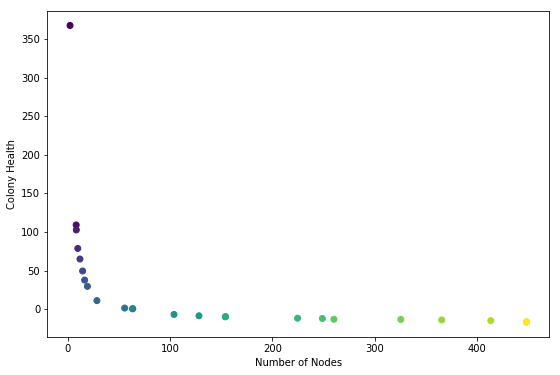
NOTE: colors are for verifying that node health ordering is correct

At first glance this was completely the reverse of what I was hoping to see. I expected to see a convex buldge pointing towards the upper right hand corner.

Hypothesis 1:

It looks as if the ea is trying to minimize the number of nodes and the colony health. This is not what the code specifies.

Hypothesis 2:

I did set up a system where high health is likely to be achived by a colony with a low number of nodes, and vice-versa. It could be that this curve, which looks like an inverse-relationship, is a result of the mechanics of the system. It might be inevitable. If that is the case I would expect to see the curve bump out generation by generation.

# Save an image for each genome in the final population
import mayavi.mlab as mlab
for i,idx in enumerate(ordered_idx):
    genome = info.final_pop[idx]
    p = ev.make_phenotype(genome)
    p.show_lines()
    mlab.savefig(str(i).zfill(2)+'_genome_'+str(idx)+'.png')
    mlab.close(all=True)

health_rank = 15
idx = ordered_idx[health_rank]
genome = info.final_pop[idx]
p = ev.make_phenotype(genome)

p.number_of_elements()

151

p.get_health()

-10.443708609271523

#print(genome)

p.show()

Below is a screen shot of the 3d view generated by show(): 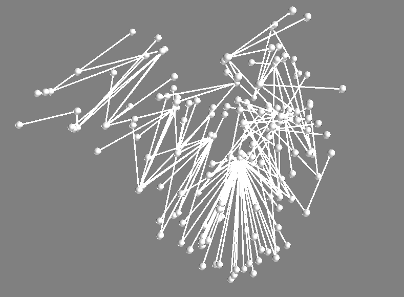It makes sense that this has low health! The nodes below are being starved for nutrients. But it has many nodes. After inspecting alot of the solutions, I think the evolution may be working right after all (looks like Hypothesis 2 is pulling ahead). Next steps are to make a compiliation of the images for all of the solutions in this final population. Edit just made this image. See the next post.

here is another one from health_rank = 9: 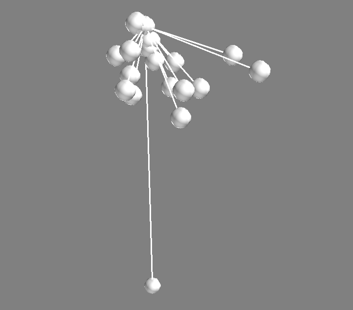(number of nodes = 24, health = 19 )

Today I spent some time understanding the knapsack example, provided by the deap documentation. This is a great example for me because it uses multi-objective optimization, which is critical for my current curiosity. More on that in a future post.

My goal was to make sure that my understanding of multi-objective optimization corresponds with what is actually possible with DEAP. Since I like visuals, I decided to make a plot of what the evolution is doing. Here it is:

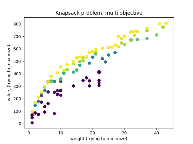
Oooh pretty colors. This plot was made using matplotlib. The color map is matplotlib.cm.viridis.

Each color represents a generation in the evolution. Brighter colors are newer generations. Each dot is an individual solution to the knapsack problem. The knapsack problem is like the problem faced by a backpacker who is trying to decide what items to put in her ‘knapsack’. There are a bunch of items with some weight and value. The goal is to have a ‘knapsack’ that is below some critical weight, and has high value. So the optimization problem has multiple objectives: low-weight and high value.

The easy way to adapt this to a normal evolutionary algorithm is to perform a weighted sum of the two objectives. The problem is that by scaling the two metrics and suming, a bias is injected into the search. Only solutions that perform well for a particular level of relative importance between the objectives will be found. This is quite limiting when you are interested in seeing a wide range of good solutions. Other problems exist with the weighted sum approach: How does one scale objectives that have unkown bounds? How does one scale objectives that have radically different meanings or units?

Luckily there is an elegant way to completely avoid cobbling disimilar metrics together. The essential idea is the pareto frontier. Basically this is the set of all individuals that are the best in their own special way at some combination of objectives (this property is called ‘non-dominated’). All the evolution has to do is select individuals from the pareto frontier, and after many generations the frontier gets better and better. See the wikipedia on multi-objective optimization.

So if we plot the weight and value for each individual, and color them by generation, we should see the dots forming a sort of buldge that moves further from the previous colors. This is indeed what we see. I was a little confused at first that the bulge moved to the upper right. This is reconciled by the fact that the algorithm is selecting for low weight.

Also, wow matplotlib’s new default plotting looks pretty good. Go open source!!

I am not really sure if this Colony Evolver project intends to be science, or art, or what. But it is clear that certain projects made by other people are very similar and exciting. Perhaps these other projects will help clear up what category this one falls into.

One such creation is described in this article about the generative design of creature sounds. A quick summary: the computer game no man’s sky contains many planets populated with a variety of creatures. Many aspects of the game are generative, which allows for a very large number of planets, each with unique terrain, creatures etc. Because the body plans of creatures are generative, the game designers decided to have the creature sounds be generative as well. The article desribes how this was done with a simulated vocal cord, resonating chamber, and mouth. A sound expert used the simulated system to make noises for archetypal creatures. It appears that these archetype sounds were modulated to fit the bodies of newly generated creatures.

You can listen to a bunch of the creatures here. What I find intriguing about this is that it certainly sounds like our idea of a swampy dinosour-inhabited ecosystem, but you can still hear hints of computer-originated noise. The bird chirps sound vaguely electronic.

For me the generative work that creates artifacts which lie on the edge between familiar and strange are the most intruguing. I am glad the bird-like chirps are slightly computer-ish. Sure, an amazing model can be created that fools the senses, but if that is the goal I would much rather experience the real thing embedded in the richness of reality.

A funny thing happened a few weeks ago. I was getting an evolution running with a fitness criteria that rewarded individual colonies for having a number of nodes close to a target number (T). I set T=13, arbitrarily.

I was using this simple fitness criteria because I wanted to ensure that evolutions were getting better, and also see if different evolution runs resulted in a variety of structures.

So I ran an evolution search for 13 node colonies, and I got structures where all but the seed nodes had location=(NaN, NaN, NaN). Of course this resulted in no appreciable strcture, so it was not visually interesting to look at. This happened because of a loop-hole in the primitive functions I had supplied to the genetic-programming framework. So I made sure no NaN values could be produced. Next run of the evolution a similar thing happened but with all zeros (location = (0, 0, 0) ).

At this point I thought to myself “whoa it is taking advantage of the system!” Without realizing I was treating the algorithm as if it had intention, as if it were a deceptive trickster. Well, certainly I had explicitly set the intention to 13 node-colonies. But I felt I was battling, or perhaps collaborating, or conversing with this entity that had intention of its own. I guess it preferred simpler solutions, all NaN’s or all zeros; more nothingness, less shape. Whereas I wanted shape, something to look at. Funny how quickly I prescribed an “intelligent” actor even though I had set up the mechanism in the first place!

This is what it looks like to run the system.

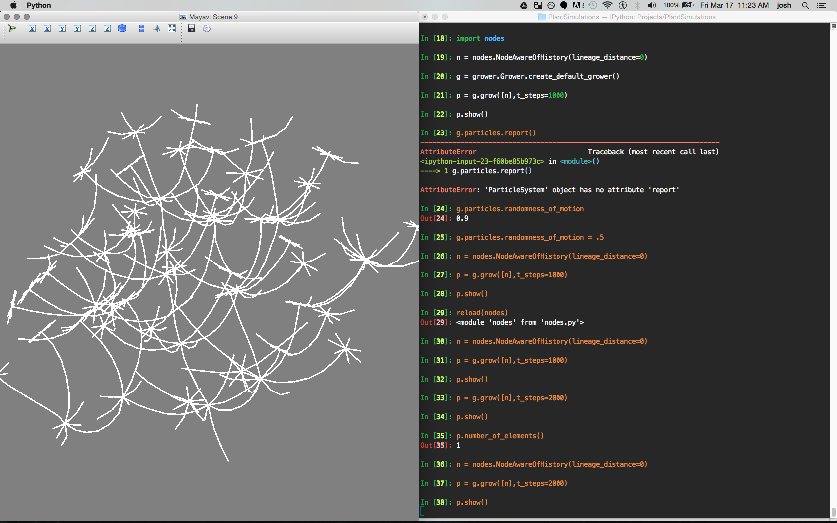
Right:

An Ipython interactive session is used to load the modules and create a grower object, a node object, and then a colony (p). The colony is grown using a seed consisting of one node [n].

Left:

The 3d visualization of the grown plant. Rendered using the mayavi library.