Multi Objective First Run
Summary
multi-objective worked and spat out a range of solutions. The solutions are on a frontier that at first sight looks not-optimal, but may be so because of the problem formulation. Skip to Fun Pictures.
This code was run and shared using jupyter. Many thanks to this post explaining how to put a jupyter session into a jekyll blog.
The evolve_colony_multi_obj.py script that generated the data is in git tag multi-obj-0.
Jupyter Session
import evolve_colony_multi_obj as ev
reload(ev)
<module 'evolve_colony_multi_obj' from 'evolve_colony_multi_obj.py'>
The imported module is a script with a main() function that runs the evolution. The fitness evaluator outputs (size, health) for the evaluated phenotype (a colony of nodes).
info = ev.main()
/Library/Frameworks/Python.framework/Versions/2.7/lib/python2.7/site-packages/transforms3d/quaternions.py:400: RuntimeWarning: invalid value encountered in divide
  vector = vector / math.sqrt(np.dot(vector, vector))


gen	nevals	avg                          	std                          	min                        	max
0  	25    	[ 179.69142857  100.03209854]	[ 158.46217436  167.08081721]	[  2.         -19.99791905]	[ 439.57142857  355.        ]
1  	48    	[ 227.76571429   16.73458574]	[ 143.79577287  101.42524822]	[  2.         -16.86966543]	[ 447.          364.64285714]
2  	46    	[ 233.31428571   17.55206654]	[ 138.30070167  102.03801106]	[  2.         -16.86966543]	[ 447.          364.64285714]
3  	45    	[ 235.76571429   20.21989035]	[ 153.93481727  102.09670425]	[  2.         -16.06184076]	[ 447.          364.64285714]
4  	39    	[ 175.50285714   38.46083977]	[ 145.44557363  120.98575388]	[  2.         -16.71785968]	[ 448.57142857  364.64285714]
5  	46    	[ 173.79428571   37.89007022]	[ 137.98761897  121.15668099]	[  2.         -16.71785968]	[ 448.57142857  364.64285714]
6  	41    	[ 190.66285714   39.57204475]	[ 147.25656566  121.45121315]	[  2.         -16.71785968]	[ 448.57142857  364.64285714]
7  	46    	[ 148.56         61.71167985]	[ 152.06825492  134.6276333 ]	[  2.         -16.71785968]	[ 448.57142857  364.64285714]
8  	45    	[ 143.56571429   87.54939393]	[ 154.78536808  156.97171347]	[  2.         -16.71785968]	[ 448.57142857  364.64285714]
9  	47    	[ 173.69714286   21.5299556 ]	[ 157.46930933   77.42182592]	[  2.         -16.71785968]	[ 448.57142857  367.85714286]
10 	46    	[ 160.92571429   27.50332923]	[ 159.32660395   79.07821019]	[  2.         -16.71785968]	[ 448.57142857  367.85714286]
n_nodes = []
health = []
for individual in info.final_pop:
    N,H = individual.fitness.values
    n_nodes.append(N)
    health.append(H)
import matplotlib.pyplot as plt
import matplotlib.cm as cm
# order by health
import numpy as np
ordered_idx = np.flip(np.argsort(health), 0)
health = np.array(health)[ordered_idx]
n_nodes = np.array(n_nodes)[ordered_idx]
v = np.linspace(0, 1, len(n_nodes))
color = cm.viridis( v )
fig = plt.figure(figsize=(9,6))
#fig = plt.figure()
plt.scatter(n_nodes, health, c=color)
plt.xlabel("Number of Nodes")
plt.ylabel("Colony Health")
plt.show(fig)
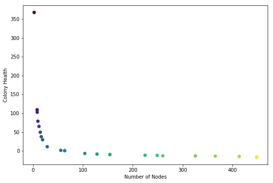
NOTE: colors are for verifying that node health ordering is correct
At first glance this was completely the reverse of what I was hoping to see. I expected to see a convex buldge pointing towards the upper right hand corner.
Hypothesis 1:
It looks as if the ea is trying to minimize the number of nodes and the colony health. This is not what the code specifies.
Hypothesis 2:
I did set up a system where high health is likely to be achived by a colony with a low number of nodes, and vice-versa. It could be that this curve, which looks like an inverse-relationship, is a result of the mechanics of the system. It might be inevitable. If that is the case I would expect to see the curve bump out generation by generation.
# Save an image for each genome in the final population
import mayavi.mlab as mlab
for i,idx in enumerate(ordered_idx):
    genome = info.final_pop[idx]
    p = ev.make_phenotype(genome)
    p.show_lines()
    mlab.savefig(str(i).zfill(2)+'_genome_'+str(idx)+'.png')
    mlab.close(all=True)
health_rank = 15
idx = ordered_idx[health_rank]
genome = info.final_pop[idx]
p = ev.make_phenotype(genome)
p.number_of_elements()
151
p.get_health()
-10.443708609271523
#print(genome)
p.show()
Below is a screen shot of the 3d view generated by show():
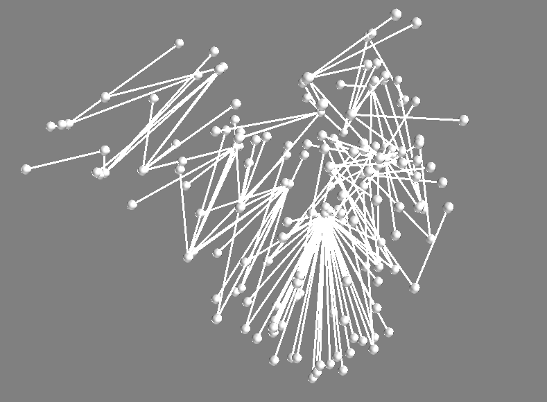 It makes sense that this has low health! The nodes below are being starved for nutrients. But it has many nodes. After inspecting alot of the solutions, I think the evolution may be working right after all (looks like Hypothesis 2 is pulling ahead). Next steps are to make a compiliation of the images for all of the solutions in this final population. Edit just made this image. See the next post.
here is another one
from health_rank = 9:
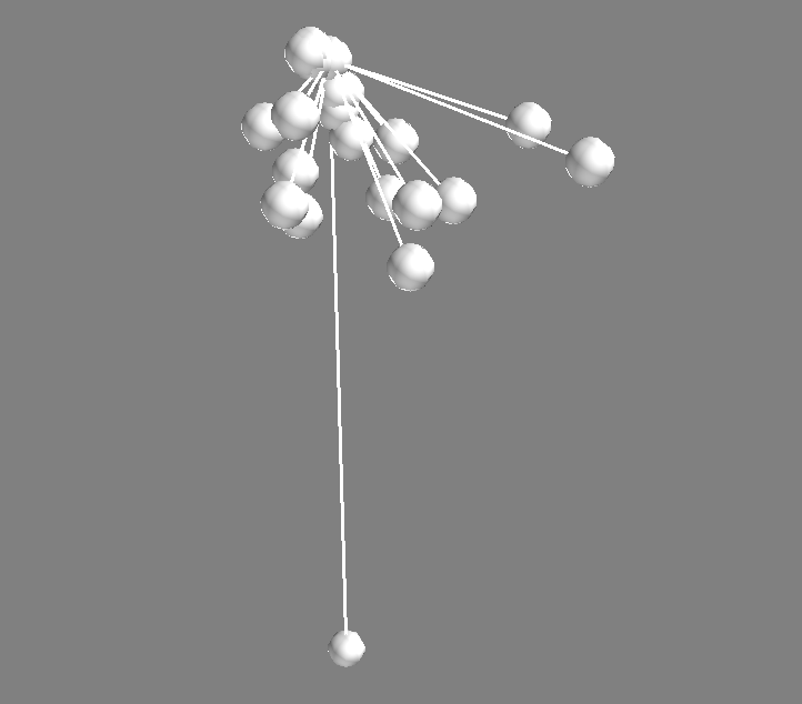 (number of nodes = 24, health = 19 )