How I Am Using Genetic Programing To Grow Shapes
This post is back-filled from my website blog. This explains how the simulation works and how genetic-programming is being used.
The Simulation
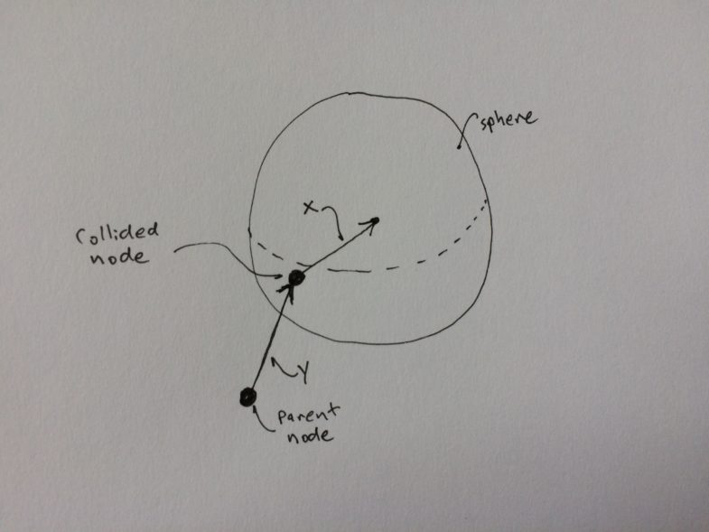
Today I got the simplest use of the genetic programming package woking: generating random trees of functions, to make a sort of ‘processor.’ I took the randomly generated processor and plugged it into the plant/coral simulation I have been developing. In this simulation a bunch of spherical particles jitter downwards, roughly simulating the diffusion of nutrients in water or light in a forest. A point, or collection of points, acts as a ‘seed.’ When a sphere collides with the seed, it creates a new point and an edge. I will refer to the points as ‘nodes.’ Each node decides where to put the child node. For the moment this decision is based on the position of the collided sphere, and it’s relative position to its parent node.
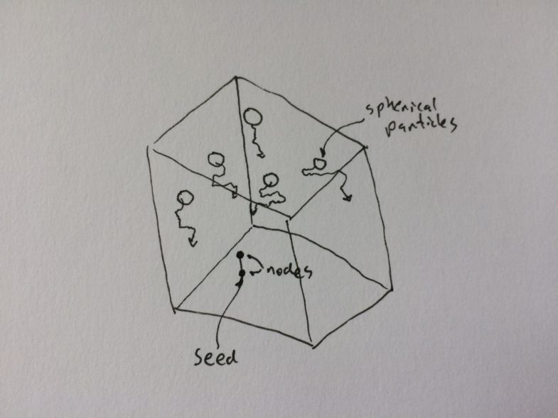
The decision of where to put the new node is where the randomly generated processor comes in. Normally I would write the program or sub-routine that decides where to put the next node. Indeed I have been doing that for a bit. But I am interested in making generative shapes that evolve! Presumably many of the plant, algae and coral shapes that we observe in the real world have growth rules that have evolved and been subjected to natural selection. Seeing all of that variation makes me want to experiment with virtual growth systems and simulated evolution. This is the first step in that direction.
How Genetic Programming Works in this Project, for the time being
There are a set of ‘primitive functions’ that are sampled randomly to create a nested series of function calls. There is also a set of ‘terminals’ which are constants and variables that act as inputs to the innermost functions. Here is an example of a randomly generated processor:
mean_vec(mean_vec(rotate_vec_np(y, y, c1), rotate_vec_np(y, y, c1)), scale(rotate_vec_np(y, y, c1), dot(x, y)))
The primitive set included mean_vec, rotate_vec_np, scale and dot. The terminal set consists of the 3d vectors x,y and the constant scalar c1.
This is most easily visualized as a tree (I did not make the code to generate processor trees or visualize them. It is all from the python package deap):
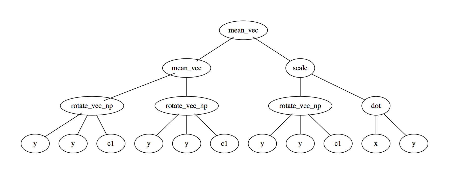
This processor tree takes in two 3d vectors and outputs a new vector. This is intentionally designed to act as the ‘decision maker’ of the node! the vector x is the relative position of the sphere to the collided node. The vector y is the vector from the parent node to the collided node.
Clearly the functions available in the primitive set, and any constants in the terminal set, are going to have an important role in constraining the possible growth behaviors. So I have been playing around with different primitive sets.
Some Randomly Generated Processor Trees and the shapes that resulted:
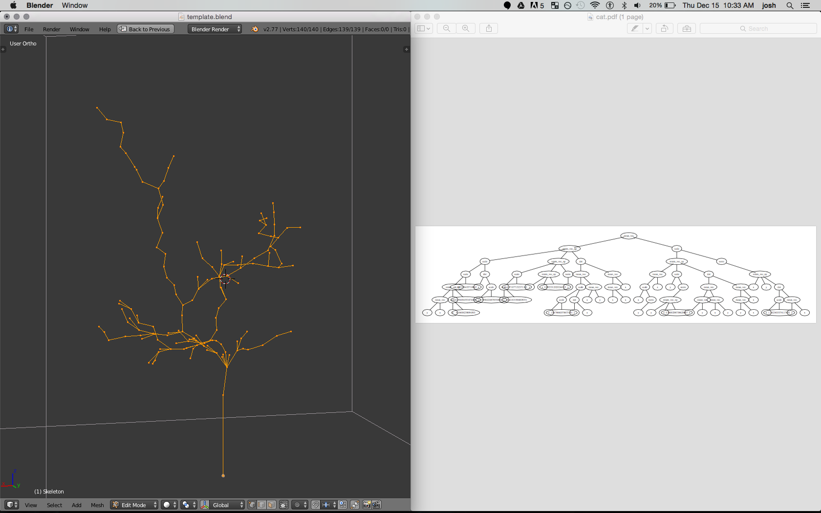
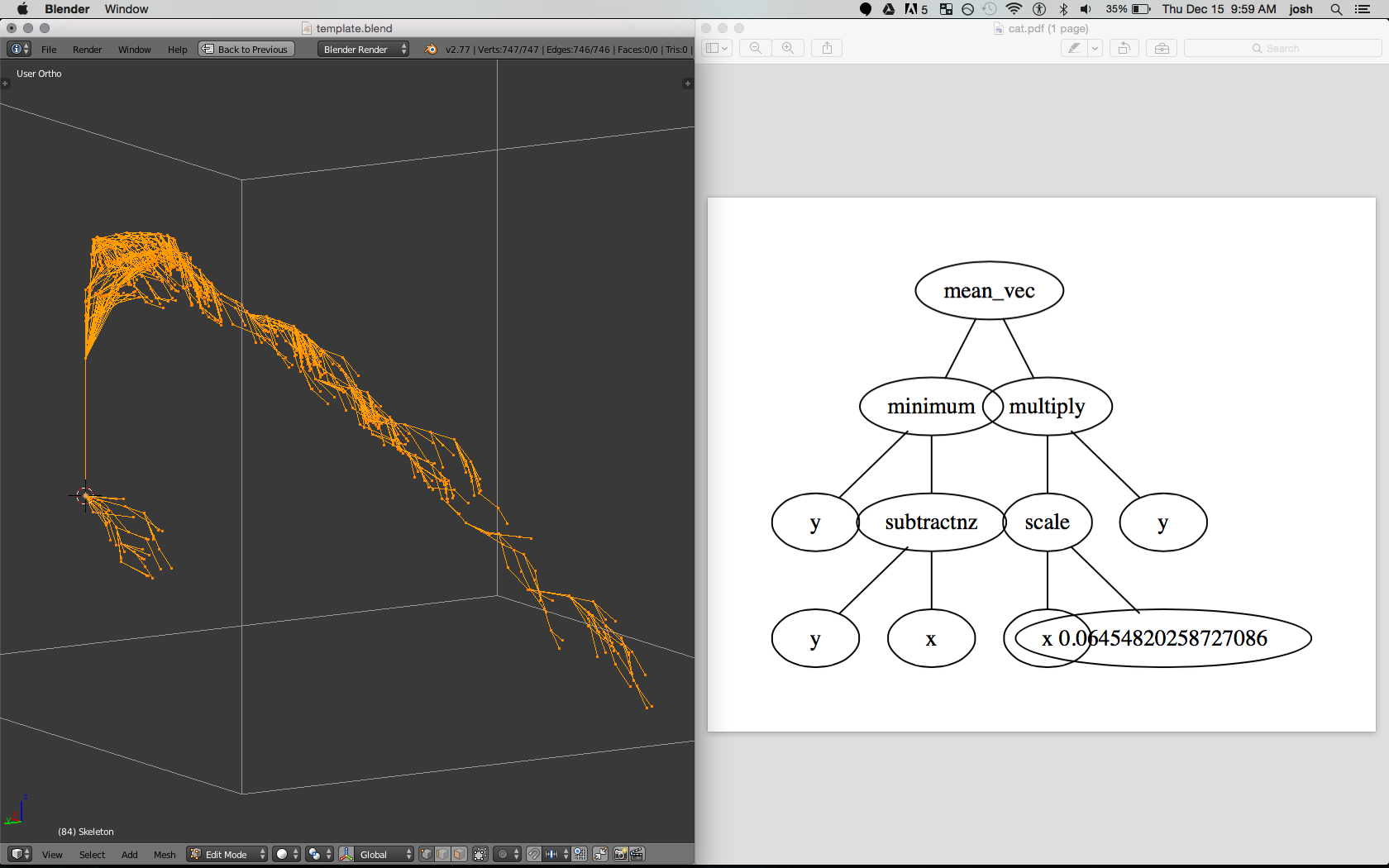
Below are some pleasing shapes that resulted (on the left), with their associated processing tree on the right.
You might notice some terminals are numbers with alot of decimals. Those are ‘ephemeral constants,’ constants that are randomly picked, in some range, when the processor was generated. Also, some of the structures are a bit lopsided. I accidentally had a setting where particles were being spawned at a side plane of the box as well as the top. In all of these cases the ‘seed’ is a line segment. This way the top most node has a non-zero vector from the parent node. If there was only one node, the y vector would be zero, and more processor trees would result in no visible structure.